Driving STEM learning effectiveness: dropout prediction and intervention in MOOCs based on one novel behavioral data analysis approach

Based on previous academic research (Xing et al., 2016; Zhang et al., 2022), it is found that STEM learning behavior is composed of timestamps, interactive learning activities, and relationships. It is used to describe a series of continuous operations that one learner performs about a certain course in the temporal sequence. All learning behavior instances are stored in logs according to the temporal order. The accuracy of dropout prediction depends on the change patterns of learning behavior distributed in the temporal sequence (Hsu, 2022), as well as the data that can be mined from it, which can provide a basis for improving the STEM learning process (Borrella et al., 2022).
In order to more accurately predict the dropout trends in the learning process, the features described by Demographic Information, Learning Accumulation, and Assessment, as well as the associated independent variables, are defined. The features are special symbols or indicators that learners or learning behavior can recognize during the learning process. For example, by using the value of highest education, the features of learners can be directly divided into “higher educated” and “low educated”, etc. At the same time, the different values of assessment results divide learners into different categories, the features of “Distinction”, “Pass”, “Fail”, and “Withdrawn” are displayed because they can be directly defined by the final results of learners. These features can be directly determined by the descriptive nature of certain attributes, known as explicit features. Additionally, based on the participation of learners in the learning process, features of learning behavior can be described as “positive” and “negative”. This is the extended description of learning behavior, but it is obtained through the calculation of learner participation and interaction frequency, the features are not direct descriptive values of attributes, but they can be derived from several other attribute values or association values, which are the implicit features. In the process of data association analysis, it is necessary to calculate all explicit features and predict associate implicit features that are used to describe the learning interests or behavior trends. However, the relationships between explicit and implicit features are externalized as specific independent variables, and latent variables can be described as different feature categories based on the values of the associated independent variables.
This study will achieve the fusion of convolutional neural networks and recurrent neural networks in the method design process. The main focus is on two aspects: (1) Convolutional neural network uses a convolutional layer, pooling layer, and fully connected layer to achieve feature extraction and classification. The convolutional layer extracts local features through convolution operations, the pooling layer is used to reduce the dimensionality of the feature map, and the fully connected layer is used for classification. Its disadvantage is that it requires normalization of all data, making it difficult to train the mixed data with different lengths, and it lacks memory function, which is definitely not conducive to data analysis and prediction of continuous learning processes. It cannot track the explicit and implicit features of learning behavior before and after dropout. (2) Recurrent neural networks are deep learning structures capable of processing sequential data. It achieves modeling and prediction of sequence data through a combination of recursive and hidden layers. The recursive layer processes the temporal relationships of sequence data through recursive operations, while the hidden layer is used to learn the representation of sequence data. Recurrent neural networks are deep learning structures capable of processing sequential data. Its disadvantage is the training complexity, which requires a large amount of labeled data, and the computational process involving multi-data structures is extremely complex. The implicit features of the learning process are mainly derived through statistics and calculations and cannot be directly labeled, so the recursive neural network cannot be used directly. In order to address the shortcomings of convolutional neural networks and recursive neural networks and to solve the problems of Fig. 1, we consider the fusion of convolutional neural networks and recursive neural networks.
The fusion method of these two neural networks mainly includes the following three steps: Step 1. Feature extraction: It involves first extracting local features from the input data through the convolutional layer, applying long short-term memory network (LSTM), and outputting them through a fully connected layer; Step 2. Feature merging: The concatenate layer achieves the association and fusion of multiple features, merging key features, and the attention mechanism is used to determine the important information of the features; Srep 3. Results output: The feature analysis results obtained in the first two steps are inputted into the recursive layer, and LSTM processes the temporal sequences with relevant state information. Finally, the analysis results of learning behavior are identified and outputted.
For the early dropout prediction process of STEM learning behavior, this study model and analyzes it in a certain temporal sequence. The relevant method is named STEM_DP. Since the dataset we selected is collected on a daily basis, the basic unit of the temporal sequence is defined as one day, which can observe more details of behavioral changes. The entire analysis process of STEM_DP is divided into four steps: firstly, we predict and select key explicit features and realize feature scoring and ranking using mutual information, random forest, and recursive feature elimination methods; secondly, we predict and mine the key implicit features of learner behavior, realize end-to-end feature tracking by constructing a convolutional neural network; thirdly, we predict and construct the topological structure of explicit and implicit features, improve the long-short-term memory mechanism of the recurrent neural network, realize the fusion with the convolutional neural network, then analyze and calculate the correlations between features and construct a learning path. Finally, combined with the analysis results of the above three steps, we derive the laws of changes in learning behavior. The analysis flow framework for dropout prediction is shown in Fig. 2.
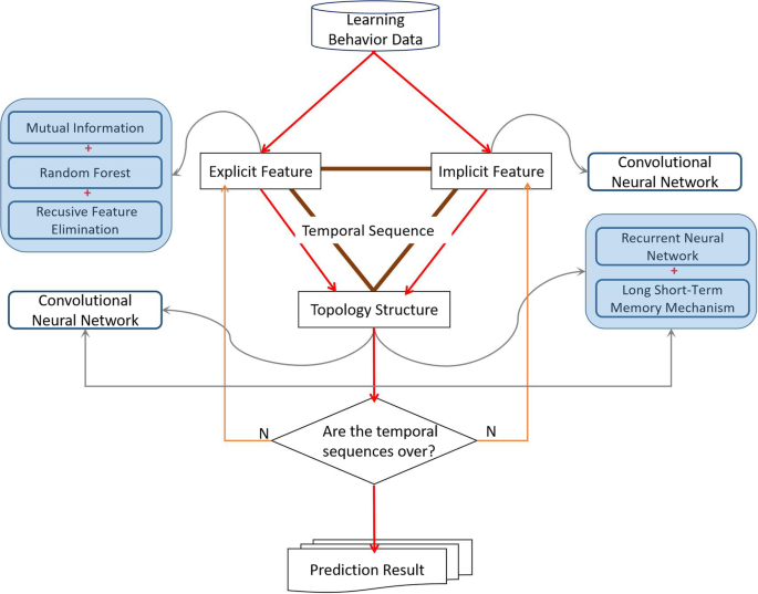
That is divided into four steps: Step 1. predict and select key explicit features and realize feature scoring and ranking; Step 2, predict and mine the key implicit features of learner behavior, realize end-to-end feature tracking; Step 3, predict and construct the topological structure of explicit and implicit features, analyze and calculate the correlations between features and construct a learning path; Step 4, derive the laws of changes in learning behavior.
The explicit and implicit features can be explored respectively by classical algorithms and convolutional neural networks. Regarding the topological structure of learning behavior, as STEM_DP combines convolutional neural network, recurrent neural network, and long-short-term memory mechanism, it needs to combine the distribution of explicit and implicit features, as well as the instance clustering in the learning process, to adopt a strategy of fusing key features and mining the strong correlation. The training process is as follows:
Step 1: The predicted results of explicit and implicit features are fused, and the related calculation formula is described as \(L_\rm T=L_\rm E+L_\rm I\) (Formula 1), where \(L_\rm T\) is the loss function of the topological structure, \(L_\rm E\) is the loss function of the explicit feature analysis process, and \(L_\rm I\) is the loss function of the implicit feature analysis process. We use cross-entropy as the loss function, defined as \(L=-\frac1m(\mathop\sum \nolimits_k=1^my_k\,\log \haty_k+(1-y_k)\log (1-\haty_k))\) (Formula 2). \(m\) is the size of the training batch, \(y_k\) is the expected output value of the \(k\rmth\) training sample in each iteration process, and \(\haty_k\) is the predicted result of the \(k\rmth\) training sample in each iteration process.
Step 2. The changes in the temporal sequence of explicit and implicit features are tracked. For the two hidden states \(h^t\) and \(s^t\) of the long short-term memory mechanism, we define the corresponding gradient values \(\delta _\rmh^t\) and \(\delta _\rms^\rmt\). The calculation formulas are described, respectively, as \(\delta _\rmh^t=\frac\partial L\partial h^t\) (Formula 3) and \(\delta _\rms^t=\frac\partial L\partial s^t\) (Formula 4), \(\delta _\rmh^t\) is jointly determined by the output gradient error for the corresponding convolution layer, i.e., \(\delta _\rmh^t=\frac\partial L\partial h^t=\frac\partial l(t)\partial h^t+\frac\partial L(t+1)\partial h^t\cdot \frac\partial h^t+1\partial h^t=V^\rm T(\haty^t-y^t)+\delta _h^t+1\cdot \frac\partial h^t+1\partial h^t\) (Formula 5). \(l(t)\) represents the loss of the \(t\rmth\) temporal sequence, \(L(\rmt+1)\) represents the loss of the temporal sequence whose time index is greater than \(t\), and \(V\) is the weight coefficient from the hidden state to the output.
Step 3. In the calculation process incorporating long short-term memory mechanism, the reverse gradient error of \(\delta _\rms^t\), denoted as \(\delta _\rmC^t\), is jointly determined by the gradient error of \(\delta _\rms^t+1\), and the gradient error obtained from \(h^t\) in the corresponding convolution layer is described as \(\delta _\rmC^t=\frac\partial L\partial s^t+1\cdot \frac\partial s^t+1\partial s^t+\frac\partial L\partial h^t\cdot \frac\partial h^t\partial s^t=s^t+1\odot f^t+1+\delta _\rmh^t\odot o^t\odot (1-\tanh ^2(s^t))\) (Formula 6), where \(f\) is the convolution function. The weight coefficients for learning route prediction can be calculated based on \(\delta _{\rmh}^t\) and \(\delta _{\rms}^t\).
Step 4. The forget gate weight coefficients of long short-term memory mechanism are defined as \(W_\rm f\). The gradient calculation formula is described as \(\frac\partial L\partial W_f=\mathop\sum \nolimits_t=1^\tau \frac\partial L\partial s^t\cdot \frac\partial s^t\partial f^t\cdot \frac\partial f^t\partial W_f=\mathop\sum \nolimits_t=1^\tau [\delta _s^t\odot s^t-1\odot f^t\odot (1-f^t)](h^t-1)^\rm T\) (Formula 7), where \(\tau\) denotes the index of the last temporal sequence and is equivalent to the length of the entire complete temporal sequence.
This computational process can help the information processing system better adapt to complex temporal data, thereby improving processing efficiency and accuracy. In this process, explicit and implicit features are merged, modeled through a topology based on the convolutional neural network. Through continuous iterative training and optimization, the information processing system is able to automatically adjust the topological relationships based on actual circumstances and learn more accurate feature representations, thus possessing better adaptability in processing temporal data.
Experiments
Based on the three STEM courses and their corresponding learning behavior instances, STEM_DP is used to test the relevant problems proposed in the section “Data standardization and problem description” and evaluate performances in predicting dropout. In order to track learners’ dropout trends, a comparative analysis of the evaluation indicators is analyzed to obtain the patterns that meet certain requirements. STEM_DP is iterated multiple times to select the optimal prediction results.
The dropout labeling for the learning behavior instances of 2013 and 2014 is as follows: Since assessment results of learners are described as four values, namely Distinction, Pass, Fail, and Withdrawn, learners labeled as Withdrawn are defined as dropouts and marked with “1”, while learners labeled with other values are considered as non-dropouts and marked with “0”. In the experimental process, the mini-batch stochastic gradient descent optimization algorithm helps to learn and select the suitable parameters, with a learning rate set at 0.001, a batch size is 256, and a total iteration set of 20,000 times. To complete the training and testing of STEM_DP, the dataset is randomly divided into training and testing sets in 8:2.
The learning behavior instances are modeled, and the four indicators of the test set are tracked and calculated. The changes in the indicator curves are visualized to explore the patterns of learning behavior. Figures 3–5 illustrate the relationships between participation and different learning periods for three STEM courses. It can be seen that the learning behavior of DDD and FFF involves four learning periods, while EEE involves three learning periods. Even for the same course, the group trends of interactive learning activities among learners vary across different learning periods. Learners’ participation is not only constrained by the courses but also by different learning periods. Therefore, dropout prediction should be implemented separately for each learning period, and performance indicators should be recorded to calculate the average values.
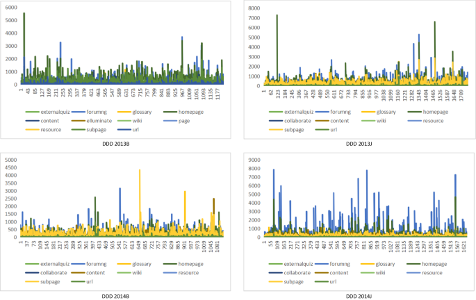
That illustrates the relationships between participation and different learning periods (including 2013B, 2023J, 2014B and 2014J) for DDD.
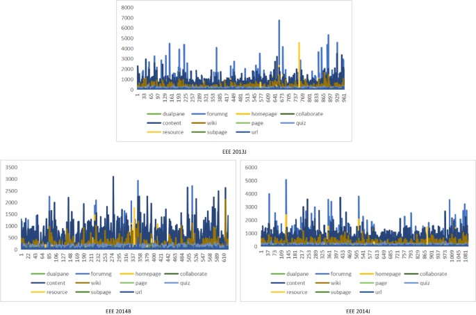
That illustrates the relationships between participation and different learning periods (including 2013J, 2014B and 2014J) for EEE.
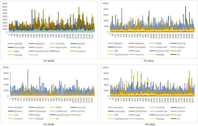
That illustrates the relationships between participation and different learning periods (including 2013B, 2013J, 2014B and 2014J) for FFF.
During the performance evaluation of STEM_DP, four indicators, Precision, Recall, F1 and AUC are selected. The dropouts of each learning period for the three courses are tracked and predicted. Thirty consecutive days are randomly selected from each period 10 times, and the average performance values of each period are calculated. Then the performance indicators of multiple learning periods for each course are averaged. Through sufficient data validation, Fig. 6 is obtained, it can be seen that the four performance indicators for the three courses are all above 0.900, indicating that the data analysis and prediction of STEM_DP have high reliability and accuracy. Among these three courses, FFF has the most types of interactive learning activities, the highest participation, and the largest scale for learning behavior. However, STEM_DP has the best data training effect, which is suitable for the associated calculation of multiple features and complex relationships, effectively tracking the temporal sequence of learning behavior, and achieving accurate classification and fusion. Since randomly 10 selected consecutive temporal sequences of 30 days are taken as the basic duration, a comprehensive analysis of the full learning process of STEM_DP is achieved.
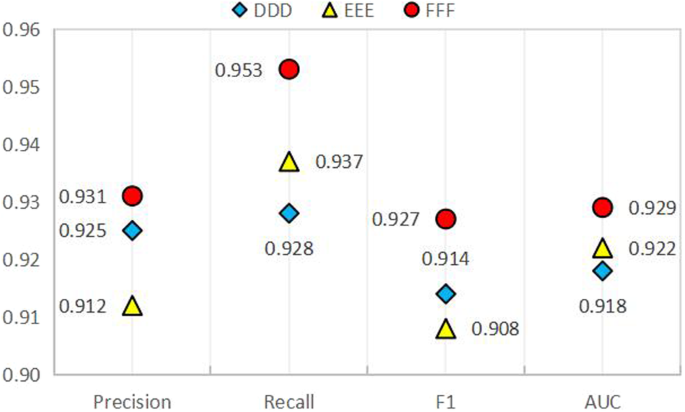
Four indicators “Precision”, “Recall”, “F1” and “AUC” are calculated and obtained for three courses “DDD”, “EEE” and “FFF”.
Furthermore, the performance change pattern of STEM_DP in the temporal sequence is tested, and the relatively optimal predictable temporal sequence is identified. Taking the learning behavior instances of three courses in 2014B as the analysis sample, 30 days are taken to form a continuous temporal sequence. STEM_DP analyzes and predicts the participation in interactive learning activities for each day, and the results of the four performance indicators are shown in Fig. 7.
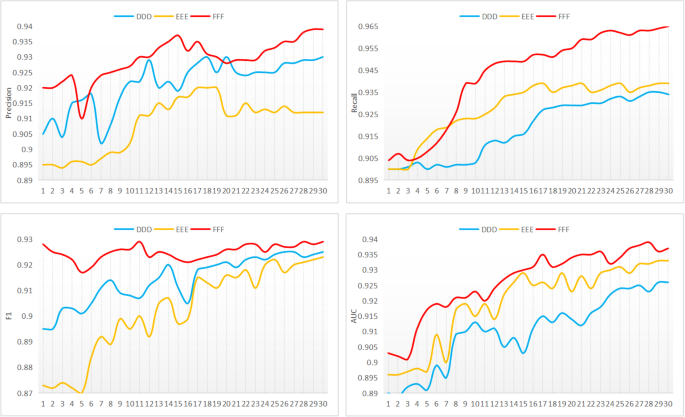
30 days are taken to form a continuous temporal sequence. With the tracking and calculation of STEM_DP, the interactive learning activities for each day are analyzed and predicted correctly.
Due to the extremely imbalanced learning behavior instances associated with DDD, EEE, and FFF, the proportion of dropout types is about 75%. The predictive performance indicators reach at least 75%, and experimental results find that these four indicators all meet the requirements. The predicted Precision for each day of the three courses exceeds 89% and demonstrates an overall increasing trend. Recall, F1, and AUC show a fluctuating slow upward trend. Based on the distribution of the four indicators in Fig. 7, it is found that the predictive performances of STEM_DP are relatively stable around the first 20 days. As days went on, the interactive learning activities also increased, which further enhanced its credibility. Therefore, the 20-day should be defined as the left boundary of the temporal sequence, and dropout prediction should be implemented, the training parameters and optimization indicators of STEM_DP dynamically might be updated and adaptively adjusted to achieve the best predictive effect.
So the application of STEM_DP in predicting dropout for the STEM courses is feasible. It can accurately track the dropout trends, analyze the temporal sequence of dropout prediction, and discover the topological path of dropout behavior and possible intervention strategies. The data analysis results can effectively be applied to the problem analysis proposed in the section “Data standardization and problem description”.
link


