Effective data selection via deep learning processes and corresponding learning strategies in ultrasound image classification

True dataset

Five networks were trained on the original dataset to classify the training data into four categories: TP, TN, FP, and FN. To assess classification consistency across the five models, we analyzed the number of images that received identical labels from all models. We observed that 8,790 benign images and 5,782 malignant images were consistently labeled by all five models forming True dataset 5. Similarly, True dataset 3 was constructed by selecting images that were labeled identically by at least three out of the five models, resulting in 9,862 benign and 6,616 malignant images. The construction of True dataset 3 and True dataset 5 ensures that the selected images have a higher level of classification agreement, thereby improving the reliability of the training process.

Experimental settings

The proposed algorithm was evaluated using ResNet101 and Vision Transformer as the original network, and the outcomes are subsequently discussed. The findings from the use of other pre-trained CNNs can be found in Supplementary Information. The True network has the same architecture as the original network, but it is a model trained with a True dataset, which is a subset of the original dataset. Table 1 shows the training data used for each network to apply the proposed method. Pre-trained networks provided by MATLAB were used, specifically ‘resnet101’ and ‘visionTransformer’ (base-16-imagenet-384). The training process was standardized across both models with common settings: the maximum of 10 epochs, the initial learning rate of 0.0001, and batch normalization statistics set to ‘moving’. When training ResNet101 in MATLAB, the input image size is \(\:224\times\:224\) pixels, with the minibatch size is 100, and the detailed conditions of the Adam optimizer are the gradient decay factor of \(\:0.9\), the squared gradient decay factor of \(\:0.999\), and the epsilon of \(\:{10}^{-8}\). The training options for the Vision Transformer in MATLAB include the input image size of \(\:384\times\:384\) pixels, the mini-batch size of 8 and the SGDM optimizer with the following details: ‘LearnRateSchedule’ set to piecewise, ‘LearnRateDropFactor’ set to 0.2, and ‘LearnRateDropPeriod’ set to 5.

All experiments were conducted using MATLAB R2022a on an NVIDIA GeForce RTX 3090 GPU processor. To ensure the consistency of the model, all networks use the average probability of the networks obtained in the last three epochs out of the maximum epoch. For average probability calculation, we use the 8 th, 9 th, and 10 th probabilities out of 10 epochs for the thyroid nodule dataset. To assess classification certainty, the original network assigns probability values to each class through a SoftMax activation function. This produces two probabilities, \(\:{p}_{O}^{B}\) and \(\:{p}_{O}^{M}\), corresponding to benign and malignant classifications, respectively. We define the classification confidence as the absolute difference between these two probabilities:

A higher confidence value indicates a more certain classification, while a lower value suggests ambiguity. If this probability difference falls below a predefined threshold \(\:{T}^{*}\), the image is considered ambiguous and is reclassified using the True network.

Figure 3 shows the histograms and cumulative distributions of class probability differences \(\:|{p}_{O}^{B}-{p}_{O}^{M}|\) in the training data. The plot titled ‘Total’ is the result of all probability differences across the five networks. The remaining five plots are the results for each representative network. The distributions that the majority of probability differences cluster around 0.9 and above. Based on this analysis, we set the threshold value \(\:{T}^{*}\) to 0.9, which led approximately 38% of the training data being reclassified. If the class probability difference of the original network in proposed methods 1 and 2 is less than 0.9, the image is considered ambiguous and reclassified using the True network. The next section will show the results of applying this reclassification strategy to representative classification models such as ResNet101 and Vision Transformer.

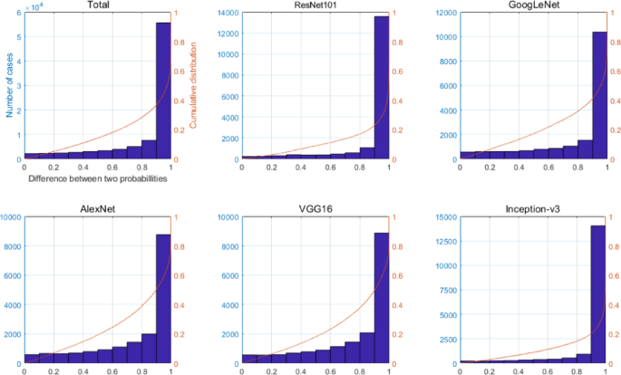
Plots with overlapping histogram and cumulative distribution of two probability differences \(\:|{p}_{O}^{B}-{p}_{O}^{M}|\) for each five representative networks used to create the True dataset. The plot titled ‘Total’ is the result of all probability differences across the five networks.

Classification results

Table 2 presents the classification results of applying the original network, the True network 3, the average method which classifies using the mean of the probabilities of these two networks, and our proposed models 1&2 in Fig. 2 to ResNet101 and Vision transformer. The classification performance of the original networks significantly differs between ResNet101 and Vision Transformer. ResNet101 exhibits a notably high accuracy of 86%, whereas Vision Transformer exhibits a comparatively lower accuracy of 73%. This discrepancy aligns with existing findings that Vision Transformer often underperform when trained on medium-sized datasets (comprising fewer than 10 million images) without robust regularization techniques in place. However, both models show performance improvements when utilizing True network 3 increases.

In particular, in the case of Vision Transformer, we succeeded in increasing the accuracy by approximately 7% compared to the original network by using only True network 3. ResNet101 showed performance improvement in the proposed models compared to the model proposed using only the True network 3. However, in the case of Vision Transformer, the proposed models did not outperform the True network 3. Nevertheless, both proposed models contribute to performance enhancement over the original network. Furthermore, examining Table S-1 (Supplementary Information), which presents the results from 11 additional CNNs, it can be observed that models utilizing both the original and true networks, such as Average and Proposed models, tend to outperform those using only the original or true networks individually.

As a result, while the Vision Transformer showed significant performance improvement with True network 3, its accuracy remains 4% lower than the best result achieved by ResNet101. Therefore, for small size of dataset of thyroid nodule ultrasound images, ResNet101 appears to be a more effective choice over the Vision Transformer. However, the results presented in this section are based solely on True Network 3. In the next section, we analyse the performance of True Network 5 and compare its effectiveness relative to True Network 3 to better understand the impact of training data size and selection strategy on classification accuracy.

Results using the other true network

Table 3 presents the results of applying True network 5 to our method. Comparing these results with those utilizing True network 3 in Table 2, it models employing True network 3 demonstrate better performance for both ResNet101 and Vision transformer compared to those utilizing True network 5. However, the observed differences depend on both the architecture and dataset characteristics. For ResNet101, the performance difference between the two True Networks is minimal, suggesting that ResNet101’s classification ability is less affected by the training subset size. In contrast, Vision transformer, which is more sensitive to the amount of training data, achieves approximately 5% higher accuracy with True network 3 trained on approximately 1,900 more images than True network 5. This result suggests that dataset size plays a more significant role in Vision Transformer’s performance than in ResNet101. Therefore, for ultrasound image classification, training True networks using True dataset 3, which includes a larger amount of data than True dataset 5, appears to be more effective in improving performance. The Grad-CAM visualizations for the original network and True network 5 using ResNet101 are presented in Fig. 4. Grad-CAM generates heatmaps highlighting the important regions used by the CNN for classification. Figure 4 depicts instances where the True network effectively classifies images with significant differences in probability compared to those misclassified or with small probability differences by the original network. While the original network trained on the entire dataset tends to focus on small parts of the nodule or areas without nodules, the True network demonstrates an overall focus on the entire nodule, potentially leading to more reliable classification.

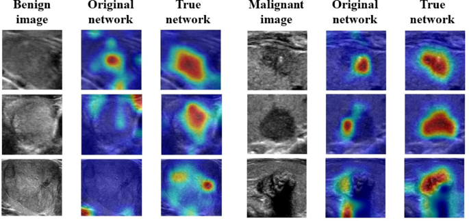
Grad-CAM visualization for ResNet101 applied to six ultrasound images (three benign and three malignant). The figure is structured in a 3 × 6 format, where the first column contains benign images, the second column shows the corresponding Grad-CAM results from the original network, and the third column presents the Grad-CAM results from the True network. Similarly, the fourth column contains malignant images, followed by Grad-CAM results from the original network in the fifth column and those from the True network in the sixth column. The color scale from red to blue represents the importance of different image regions, where red indicates the most critical areas used for classification. The selected images include cases where the original network misclassified or had a small probability difference, whereas the True network provided correct classification with a higher probability difference.

Modifications

This section extends the previous experiments by introducing False networks, which are trained on False datasets comprising misclassified images. With the goal of improving the performance of the original network, we employed the True network, which was trained using accurately classified images. Similarly, we aimed to apply this technique to the proposed model by generating, so-called, a false dataset through the collection of poorly classified images.

Initially, we created a false dataset by gathering images that the five pre-trained networks were unable to classify effectively. Five false datasets were constructed based on the number of pre-trained networks that classified images with the same label (FP or FN). False dataset 1 consisted of images classified as FP or FN by any of the five networks. False datasets 2–5 were similarly created. The number of ultrasound images in False datasets 1–5 were (1657,1378), (953,823), (585,544), (283,331), and (74,99) for FP or FN, respectively. In the experimental setting, False dataset 3 is chosen for use because there is a scarcity of images that receive unanimous classification as false from all five networks. Next, we trained a network with the same architecture and training options as the original network for the False dataset 3. A network trained on the false dataset 3 is called a False network 3.

The proposed algorithm depicted in Fig. 2 utilizes the True network classification result if the difference in probabilities between classes of the original network is less than 0.9 (\(\:\left|{p}_{O}^{B}-{p}_{O}^{M}\right|<0.9\)). To further enhance classification performance, we introduced an additional condition: if the final probability difference between \(\:{p}^{B}\) and \(\:{p}^{M}\)of the proposed method was less than 0.1, the image was classified once more using False network 3. The threshold of 0.1 was selected based on experimental evaluations ranging from 0.1 to 0.9, with 0.1 yielding the best results.

Experiments were implemented using ResNe101 architecture and on the False dataset 3, and the results were illustrated in Table 4. After analyzing the results, we can deduce that incorporating false data into the learning process in order to prevent networks from making incorrect decisions, by teaching them something that may not be accurate due to the inclusion of unreliable data, does not effectively enhance the performance of the networks. This suggests that False networks may not provide the same level of beneficial correction as True networks and that training on correctly classified images remains the more effective strategy for improving classification accuracy.

Result for skin cancer image dataset

To assess the applicability of the proposed technique, in this section, we examine the outcomes obtained by applying our method to classify images of melanoma, a form of skin cancer, rather than ultrasound images. Melanoma is an aggressive form of skin cancer that originates in the melanocytes and can rapidly metastasize, making early detection and accurate diagnosis critical³⁸. Since the development of deep learning, various classification methods using CNN have been developed for melanoma lesion images. The International Skin Imaging Collaboration (ISIC) Archive provides skin lesion dermoscopic images for research³⁹. ISIC provides high-resolution dermoscopic images, which minimize artifacts such as shadows and light reflections, allowing for more reliable image-based classification^40,41. For our experiment, we used a subset of the ISIC Challenge dataset^42,43, specifically selecting images labeled as benign nevi and malignant melanoma. There are 12,875 benign and 4,522 malignant images, so 10% of them are separated as test data (B:1,287, M:452). The training dataset is created by randomly selecting 4,070 images of each class from each class to ensure balanced distribution. When learning the original network for melanoma data, the data augmentation method was not used because the number of images for each class in the training data was the same.

Since the training data is very small at about 8,000 pieces, this data set was chosen as True dataset 3, which has more data than True dataset 5. True dataset 3 has 3,914 benign and 3,684 malignant images. True dataset 5 has 3,264 benign and 2,801 malignant images. Augmentation was performed to make fewer malicious images equal to benign images. The training options are the same as the training options for thyroid nodule images except that the max epoch is set to 20. Because dermoscopic images are color images, unlike grayscale ultrasound images, extending the number of epochs was necessary to allow the network to better capture relevant features. Consequently, the probability values of each network used in the experiment was the average of the probabilities of the last three networks among the entire epoch, so the 18, 19, and 20 networks were used.

Table 5 shows the results of applying the proposed method to ResNet101 and Vision Transformer for melanoma classification. The proposed models obtained by fine-tuning the ResNet101 architecture leveraging True network 3 showed improved accuracy compared to the original network. Conversely, Vision Transformer performed better with True network 5, though its sensitivity for detecting malignant cases remained low, limiting its practical applicability. To further validate the effectiveness of our proposed methods, we extend our evaluation to 11 additional pre-trained architectures beyond ResNet101 and Vision Transformer. The results are presented in Supplementary Table S-2. When using True network 3, proposed model 1 achieves higher accuracy than the original network in 10 out of 11 cases (90.9%) and outperforms True network 3 alone in 10 cases. Similarly, proposed model 2 surpasses the original network in 10 out of 11 cases, though it shows improvements over the average of the original and True network in only 3 cases. Furthermore, in 7 out of 11 architectures, proposed model 2 performs better than proposed model 1 which suggests that the averaging-based approach can be beneficial in some scenarios. When using True network 5, a similar trend was observed. The proposed model 1 shows superior accuracy over the original network in 9 out of 11 cases (81.8%) and surpasses True network 5 alone in all 11 cases. Likewise, proposed model 2 outperforms the original network in 11 cases and exceeds the average of the original and True network in 11 cases, showing a more consistent improvement. Additionally, proposed model 2 performs better than proposed model 1 in 9 out of 11 architectures and reinforces the effectiveness of probability averaging when True network 5 is used.

These findings suggest that while the True network alone does not always surpass the original network, integrating it into the proposed decision-making framework leads to consistent performance gains. Furthermore, the comparative results between proposed models 1 and 2 indicate that different network architectures may benefit more from either direct correction (proposed model 1) or probability averaging (proposed model 2), depending on the dataset and model characteristics.