
An effective study on the diagnosis of colon cancer with the developed local binary pattern method

This section details the methodologies employed in this study for colorectal cancer diagnosis, encompassing the proposed feature extraction techniques, machine learning classifiers, and transfer learning models. The framework integrates both novel and established Local Binary Pattern (LBP) variants with traditional machine learning and deep learning paradigms.
Traditional image enhancement techniques
Local binary pattern (LBP)
The Local Binary Pattern (LBP) method is a widely employed technique for texture feature extraction, favored for its computational simplicity and robustness to illumination variations. It effectively mitigates grayscale shifts caused by changing lighting conditions, making it suitable for texture analysis in image processing32,33.
The fundamental LBP operator compares the intensity of a central pixel (Pc) with its P neighboring pixels on a circular neighborhood defined by radius R. The result is an 8-bit binary number for a 3 × 3 neighborhood (P = 8, R = 1). The standard LBP calculation is defined as:
$$\:s\left(x\right)=\left|\genfrac{}{}{0pt}{}{1,\:\:\:if\:{P}_{x}>P}{0,\:\:otherwise}\right.$$
$$\:LBP=\sum\:_{x\in\:\text{1,8}}s\left(x\right).{2}^{x-1}$$
Where s(x) is defined as: s(x) = 1 if x ≥ 0 s(x) = 0 if x < 0.
Step local binary pattern (n-LBP)
Building upon the classical LBP, this study utilizes a high-performance variant known as step LBP (n-LBP)34. Unlike standard LBP, which compares each surrounding pixel directly to the central pixel, n-LBP performs pairwise comparisons between surrounding pixels in a specific order, determined by a step parameter.

Sub-image enhanced by step-LBP algorithm.
If the step parameter is one, \(\:{P}_{0}\) pixel with \(\:{P}_{1}\) pixel, \(\:{P}_{1}\) pixel with \(\:{P}_{2}\) pixel, \(\:{P}_{2}\) pixel with \(\:{P}_{3}\) pixel, \(\:{P}_{3}\) pixel with \(\:{P}_{4}\) pixel, \(\:{P}_{4}\) pixel with \(\:{P}_{5}\) pixel, \(\:{P}_{5}\) pixel with \(\:{P}_{6}\) pixel, \(\:{P}_{6}\) pixel with \(\:{P}_{7}\) pixel, and at last \(\:{P}_{7}\) pixel is compared with \(\:{P}_{0}\) pixel. This is done for n = 2, n = 3, and n = 4 as follows.
If the step parameter is two, then Pc = S(P0 > P2), S(P1 > P3), S(P2 > P4), S(P3 > P5), S(P4 > P6), S(P5 > P7), S(P6 > P0), S(P7 > P1) relation is performed.
If the step parameter is three, then Pc = S(P0 > P3), S(P1 > P4), S(P2 > P5), S(P3 > P6), S(P4 > P7), S(P5 > P0), S(P6 > P1), S(P7 > P2) relation is performed.
If the step parameter is four, then Pc = S(P0 > P4), S(P1 > P5), S(P2 > P6), S(P3 > P7), S(P4 > P0), S(P5 > P1), S(P6 > P2), S(P7 > P3) relation is performed.
Thus, some changes were introduced in the classical LBP calculation;
$$\:S\left({P}_{i}>{P}_{j}\right)=\left\{\begin{array}{c}1\\\:0\end{array}\right.\:\:\:\:if\:\:\:\begin{array}{c}{P}_{i}>{P}_{j}\\\:{P}_{i}\le\:{P}_{j}\end{array}$$
(1)
was recalculated.
Considering the sub-image in Fig. 1 above as an example, the binary equivalent of step 1:
Pc = S(36 > 221), S(221 > 129), S(129 > 80), S(80 > 145), S(145 > 190), S(190 > 219), S(219 > 168), S(168 > 36) = 01100011; the decimal equivalent of the obtained value is 99.
Considering the sub-image in Fig. 1 above as an example, the binary equivalent of step 2:
Pc = S(36 > 129), S(221 > 80), S(129 > 145), S(80 > 190), S(145 > 219), S(190 > 168), S(219 > 36), S(168 > 221) = 01000110; the decimal equivalent of the obtained value is 70.
Considering the sub-image in Fig. 1 above as an example, the binary equivalent of step 3:
Pc = S(36 > 80), S(221 > 145), S(129 > 190), S(80 > 219), S(145 > 168), S(190 > 36), S(219 > 221), S(168 > 129) = 01000101; the decimal equivalent of the obtained value is 69.
Considering the sub-image in Fig. 1 above as an example, the binary equivalent of step 4:
Pc = S(36 > 145), S(221 > 190), S(129 > 219), S(80 > 168), S(145 > 36), S(190 > 221), S(219 > 129), S(168 > 80) = 01001011; the decimal equivalent of the obtained value is 75.
Developed cross-over local binary pattern (CO-LBP)
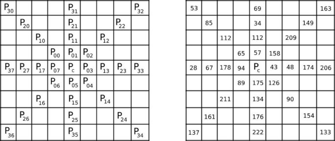
This study introduces a novel LBP variant, Cross-Over LBP (CO-LBP), designed to enhance feature extraction for histopathological image analysis. CO-LBP operates on a 3 × 3 neighborhood by comparing each of the 8 surrounding pixels with the pixel located diametrically opposite (180 degrees) to it, relative to the central pixel. This approach aims to capture radial symmetry and distinctive textural patterns inherent in histopathological structures. The architectural structure of the CO-LBP method is visually represented in Fig. 2.

The architecture of CO-LBP method.
As a result of the comparison process, an 8-digit binary number is obtained. The base 10 equivalent of the resulting number is assigned as the center pixel value. The Figure … shows the sub-image discussed and the comparison result. The formula for the CO-LBP method is shown in the formula below.
$$\:CO-LBP=\:\sum\:_{i=0}^{P}c({P}_{i}-{P}_{c}){2}^{t}$$
(2)
According to the formula above, the comparison process proceeds as follows. In the CO-LBP method, if the radius value varies between 1 and 4, the pattern solution obtained for a representative image section shown in Fig. 3.
Pixels of sample sub-image.
If the cross-over parameter is one, then Pc = S(\(\:{P}_{00}>{P}_{04}\)), S(\(\:{P}_{01}>{P}_{05}\)), S(\(\:{P}_{02}>{P}_{06}\)), S(\(\:{P}_{03}>{P}_{07}\)), S(\(\:{P}_{04}>{P}_{00}\)), S(\(\:{P}_{05}>{P}_{01}\)), S(\(\:{P}_{06}>{P}_{02}\)), S(\(\:{P}_{07}>{P}_{03}\)) relation is performed.
If the cross-over parameter is two, then Pc = S(\(\:{P}_{10}>{P}_{14}\)), S(\(\:{P}_{11}>{P}_{15}\)), S(\(\:{P}_{12}>{P}_{16}\)), S(\(\:{P}_{13}>{P}_{17}\)), S(\(\:{P}_{14}>{P}_{10}\)), S(\(\:{P}_{15}>{P}_{11}\)), S(\(\:{P}_{16}>{P}_{12}\)), S(\(\:{P}_{17}>{P}_{13}\)) relation is performed.
If the cross-over parameter is three, then Pc = S(\(\:{P}_{20}>{P}_{24}\)), S(\(\:{P}_{21}>{P}_{25}\)), S(\(\:{P}_{22}>{P}_{26}\)), S(\(\:{P}_{23}>{P}_{27}\)), S(\(\:{P}_{24}>{P}_{20}\)), S(\(\:{P}_{25}>{P}_{21}\)), S(\(\:{P}_{26}>{P}_{22}\)), S(\(\:{P}_{27}>{P}_{23}\)) relation is performed.
If the cross-over parameter is one, then Pc = S(\(\:{P}_{30}>{P}_{34}\)), S(\(\:{P}_{31}>{P}_{35}\)), S(\(\:{P}_{32}>{P}_{36}\)), S(\(\:{P}_{33}>{P}_{37}\)), S(\(\:{P}_{34}>{P}_{30}\)), S(\(\:{P}_{35}>{P}_{31}\)), S(\(\:{P}_{36}>{P}_{32}\)), S(\(\:{P}_{37}>{P}_{33}\)) relation is performed.
if the cross-over parameter is one, then Pc = S(65 > 126), S(57 > 175), S(158 > 89), S(43 > 94), S(126 > 65), S(175 > 57), S(89 > 158), S(94 > 43) = (00101101)2; the decimal equivalent of the obtained value is 45.
if the cross-over parameter is two, then Pc = S(112 > 90), S(112 > 134), S(209 > 211), S(48 > 178), S(90 > 112), S(134 > 112), S(211 > 209), S(178 > 48) = (10000111)2; the decimal equivalent of the obtained value is 139.
if the cross-over parameter is three, then Pc = S(85 > 154), S(34 > 176), S(149 > 161), S(174 > 67), S(154 > 85), S(176 > 34), S(161 > 149), S(67 > 174) = (00011110)2; the decimal equivalent of the obtained value is 30.
if the cross-over parameter is four, then Pc = S(53 > 133), S(69 > 222), S(163 > 137), S(206 > 28), S(133 > 53), S(222 > 69), S(137 > 163), S(28 > 206) = (00111100)2; the decimal equivalent of the obtained value is 60.
Comparative analysis with symmetric and Rotation-Invariant LBP variants
To contextualize the novelty of CO-LBP, a theoretical comparison with established LBP variants is presented in Table 1. Standard LBP compares the center pixel to neighbors, lacking inherent symmetry handling or rotation invariance. Rotation-Invariant LBP (RI-LBP) achieves orientation independence through circular bit shifts but may lose discriminative features15,35,36. Symmetric LBP variants (e.g., CS-LBP) compare adjacent pairs, potentially overlooking radial patterns critical in glandular structures16,37.
In contrast, CO-LBP’s 180° opposite pixel comparison naturally encodes radial symmetry without post-processing, preserves discriminative power, aligns with glandular architecture, and maintains computational efficiency (O(n)). This design rationale positions CO-LBP as particularly suited for histopathological analysis.
Deep convolutional feature extraction
To evaluate the efficacy of LBP-derived features within a deep learning context, five representative deep convolutional neural network architectures were selected, encompassing various design paradigms: Residual Learning (ResNet50, ResNet101), Dense Connectivity (DenseNet201), Mobile Optimization (MobileNet), and Compound Scaling (EfficientNetV2). Subsequent analysis focuses primarily on ResNet50 and MobileNet, as they effectively demonstrate the accuracy-efficiency trade-off pertinent to clinical deployment.
ResNet50
The ResNet50 architecture is characterized by its residual learning blocks (ResBlocks), which enable the training of very deep networks by learning residual functions38. This design mitigates the vanishing gradient problem, facilitating the optimization of deeper networks. ResNet50 comprises 50 layers and typically accepts input images of size 224 × 224 × 338.
ResNet101
ResNet101 extends the residual learning concept of ResNet50, featuring 101 layers38,39. It employs the same residual optimization principle to minimize parameters and mitigate the impact of increased depth on performance, allowing for potentially more complex feature extraction.
EfficientNetV2
EfficientNetV2 is an evolution of the EfficientNet architecture, prioritizing parameter efficiency and training speed without sacrificing accuracy39,40,41. It incorporates fused early layers, prefers smaller expansion ratios and kernel sizes, and adjusts layer configurations to optimize performance40,41,42.
DenseNet201
DenseNet201 improves gradient flow compared to ResNet by directly connecting each layer to all preceding layers within a dense block. This connectivity enhances feature propagation and encourages feature reuse, often leading to models with fewer parameters and high performance on image classification tasks42,43.
MobileNet
MobileNet is a lightweight convolutional neural network designed for mobile and embedded vision applications. It utilizes depthwise separable convolutions to significantly reduce computational cost and model size, making it suitable for resource-constrained environments44.
Machine learning algorithms
Following LBP feature extraction, various machine learning algorithms were employed for classification within the WEKA 3 software45 environment.
Decision table
The Decision Table algorithm provides a structured method for classification by storing feature-value combinations and their associated class labels46. It offers a transparent and interpretable approach to decision-making, functioning on an “If., then.” logical structure46.
IBk (K-nearest neighbors)
The IBk algorithm in WEKA implements the K-Nearest Neighbors (KNN) method47. It classifies a sample based on the majority class among its k nearest neighbors in the feature space, defined by a distance metric47.
Optimized forest
The Optimized Forest algorithm is a genetic algorithm-based ensemble method derived from the decision forest approach. It aims to enhance overall accuracy by evolving a population of decision trees, selecting those with high accuracy and diversity through genetic operations like crossover and mutation, guided by an elitist selection strategy48.
Random forest
Random Forest is an ensemble learning method that combines multiple decision trees to improve predictive accuracy and control overfitting48. It builds trees using bootstrap samples of the data and considers only a random subset of features at each split, reducing correlation between individual trees48.
Resample
The Resample algorithm generates random subsamples of the dataset, either with or without replacement, to create new training sets48,49,50. It was used in this study for data preprocessing, particularly to address potential class imbalances.
Smote
The Synthetic Minority Oversampling Technique (SMOTE) generates synthetic examples of minority classes by interpolating between existing instances. This technique helps balance class distributions in the dataset, potentially improving classifier performance on minority classes49.
link


