The innovation path of VR technology integration into music classroom teaching in colleges and universities

Principle and implementation process of IIMT model construction

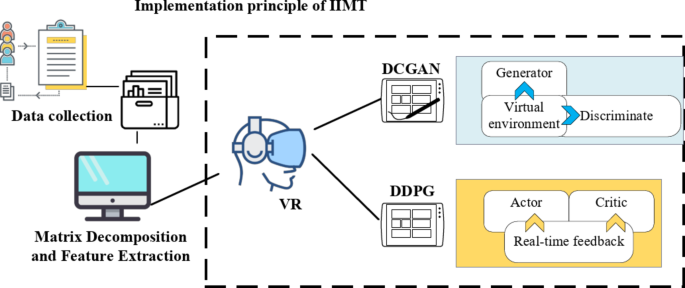
This study proposes the Intelligent Interactive Music Teaching (IIMT) model, which integrates VR technology, DCGANs, and the DDPG reinforcement learning algorithm. The objective is to enhance immersion, interactivity, and personalization in music education. DCGANs are employed to generate high-quality virtual music teaching environments. The generator extracts and synthesizes high-dimensional images and audio relevant to the instructional context using multi-layer convolutional neural networks, progressively refining detail and visual quality. The discriminator then applies adversarial training to assess and enhance the realism and educational relevance of the generated content. This iterative process ensures that the virtual environments closely resemble real-world teaching scenarios, thereby improving immersion. Simultaneously, the DDPG algorithm dynamically adjusts student interactions and feedback in real-time to optimize teaching strategies. DDPG integrates policy gradient methods with deep learning and consists of two key components: the policy network (Actor) and the value network (Critic). The Actor selects appropriate teaching actions based on student interactions, while the Critic evaluates their effectiveness and refines the Actor’s decisions through a feedback mechanism. This approach allows the system to manage the continuous action space inherent in music education, modifying instructional difficulty and adapting virtual environments according to students’ progress and feedback^27,28,29. By doing so, the system personalizes learning pathways, ensuring that students receive instruction suited to their individual needs³⁰. In this integrated model, VR technology provides an interactive platform for the virtual environments generated by DCGANs, while the DDPG algorithm continuously refines these environments and teaching strategies based on real-time student data. This process creates a dynamic feedback loop in which adversarial training and reinforcement learning collectively enhance both the virtual learning experience and instructional effectiveness. Figure 1 illustrates the operational framework of the IIMT model.

Implementation principle of IIMT model.

Techniques and algorithms involved in the construction of IIMT model

VR technology and DCGAN algorithm

The implementation of VR technology involves several essential components, including image rendering, spatial tracking, and real-time interaction. VR systems utilize head-mounted displays and motion sensors to track users’ movements and positions, which are then updated within the virtual environment in real time. By engaging visual, auditory, and haptic senses, VR creates an immersive three-dimensional experience generated by computer simulation.

DCGANs are employed to generate high-quality images through adversarial training between two neural networks: the generator and the discriminator. The generator aims to create realistic images that can deceive the discriminator, while the discriminator attempts to differentiate between real and synthesized images³¹. This adversarial process improves the generator’s ability to capture complex image structures and features more effectively than traditional models³².

The image generation process begins with the generator \(\:G\), which receives an input noise vector \(\:z\). The generator processes this input through a multi-layer CNN to produce a visually coherent output. The mathematical formulation for the generator is given in Eq. (1):

In Eq. (1), \(\:{W}_{g1}\), \(\:{W}_{g2}\), and \(\:{W}_{g3}\) are the weights, and \(\:{b}_{g1}\), \(\:{b}_{g2}\) and \(\:{b}_{g3}\) are the biases for the generator layers. The \(\:\sigma\:\) function represents the activation function, and \(\:BN\) denotes batch normalization. To further optimize the generator, DCGAN introduces batch normalization to stabilize the training process and accelerate convergence. Batch normalization helps mitigate the internal covariate shift by normalizing the data at each layer. The specific formula for batch normalization is shown in Eq. (2):

\(\:\mu\:\) and \(\:{\sigma\:}^{2}\) are the mean and variance of the mini-batch data, respectively; \(\:B\) is a constant to prevent division by zero; \(\:\gamma\:\) and \(\:\beta\:\) are learnable parameters that scale and shift the normalized data.

The discriminator \(\:D\) receives the input image \(\:x\) and determines whether the image is real or fake using a CNN. The calculation for the discriminator is as follows:

In Eq. (3), \(\:{W}_{d1}\), \(\:{W}_{d2}\), and \(\:{W}_{d3}\) are the weights, and \(\:{b}_{d1}\), \(\:{b}_{d2}\) and \(\:{b}_{d3}\) are the biases for the discriminator layers. Leaky ReLU is employed to avoid the vanishing gradient problem, which occurs when neurons are “dead” in ReLU activation functions.

To improve the effectiveness of adversarial training, optimizing the loss functions of both the generator and the discriminator is crucial. The goal is to enhance the generator’s ability to produce realistic images while enabling the discriminator to accurately differentiate between real and generated images.

The loss function for the discriminator is defined as follows in Eq. (4):

In Eq. (4), \(\:{p}_{data}\left(x\right)\) represents the true data distribution, and \(\:{p}_{z}\left(z\right)\) denotes the noise distribution. This function ensures that the discriminator learns to differentiate between real and generated images effectively.

The generator’s loss function is given by Eq. (5).

Equation (5) guides the generator in producing more realistic images by reducing the likelihood that the discriminator correctly identifies them as fake, thereby improving the overall quality of the generated outputs.

During the optimization process, it is also crucial to update the discriminator’s weights to enhance its ability to distinguish between real and generated images. The discriminator aims to minimize \(\:{L}_{D}\), and its weights are updated using the gradient descent method as follows:

In Eq. (6), \(\:{\eta\:}_{d}\) represents the learning rate of the discriminator. According to this equation, the discriminator’s weights are updated in the opposite direction of the gradient, reducing the loss function \(\:{L}_{D}\) and improving its ability to distinguish between real and generated images.

This adversarial process allows the generator to create increasingly realistic images while the discriminator continuously refines its classification accuracy. As a result, the model enhances image generation quality and improves training efficiency.

In DCGAN, the generator and discriminator interact through adversarial training to produce high-quality images. The computational complexity of this process is primarily influenced by convolution operations and batch normalization mechanisms. The generator progressively extracts features through multiple convolutional layers, transforming the input noise vector into high-dimensional images. The complexity of each convolution operation depends on factors such as the kernel size, feature map dimensions, and the number of output channels. The discriminator evaluates image authenticity by compressing multi-layer feature maps, while batch normalization stabilizes training by computing the mean and variance of mini-batch data. However, these operations introduce additional computational overhead. During the alternating optimization of the generator and discriminator, the backpropagation of the loss function further increases computational demands. To manage this complexity, DCGAN optimizes network depth, adjusts feature map sizes, and carefully selects parameters such as batch size and learning rate. These strategies enable DCGAN to generate high-quality images while maintaining computational efficiency for real-time virtual music teaching environments.

Reinforcement learning algorithm based on DDPG

DDPG integrates the strategy gradient method with deep learning, utilizing DNNs to model both the Actor and Critic components. The Actor selects the optimal action based on the current state, while the Critic evaluates the corresponding action value. A key advantage of DDPG is its ability to enhance learning efficiency and stability through experience replay and target network stabilization^33,34.

In the initial step, the Actor generates an optimal action \(\:a\) for a given state \(\:s\). This process is represented by a deep neural network, with its computation defined in Eq. (7):

In Eq. (7), \(\:{W}_{\mu\:1}\), \(\:{W}_{\mu\:2}\), \(\:{W}_{\mu\:3}\), \(\:{b}_{\mu\:1}\), \(\:{b}_{\mu\:2}\) and \(\:{b}_{\mu\:3}\) are the weights and biases of the Actor network. This architecture enables the Actor to effectively extract features from the input state and generate corresponding actions.

Next, the Critic network evaluates the value of a given state-action pair (\(\:s\), \(\:a\)). The Critic’s computation is expressed as Eq. (8):

In Eq. (8), \(\:{W}_{Q1}\), \(\:{W}_{Q2}\), \(\:{W}_{Q3}\), \(\:{b}_{Q1}\), \(\:{b}_{Q2}\) and \(\:{b}_{Q3}\) are the weights and biases of the Critic network, and \(\:[s;a]\) represents the concatenated vector of state and action. This structure enables the Critic to effectively integrate state and action information for accurate value estimation^35,36.

To optimize the Actor and Critic networks during training, it is necessary to define their respective loss functions. The loss function for the Critic is given by Eq. (9):

In Eq. (9), \(\:Dt\) refers to the experience playback buffer, \(\:r\) is the discount factor., and \(\:\gamma\:\) denotes the discount factor. The symbols \(\:{Q}^{{\prime\:}}\) and \(\:{\mu\:}^{{\prime\:}}\) denote the target Critic and target Actor networks, respectively. The target value \(\:y\) is calculated as Eq. (10):

The loss function for the Actor network is defined as Eq. (11):

Equation (11) encourages the Actor to generate actions that maximize the Q-value.

During optimization, the weights of the Actor and Critic networks must be updated iteratively. The update equation for the Critic network is shown in Eq. (12):

Equation (12) can be further developed as:

In Eq. (13), \(\:{\eta\:}_{Q}\) is the Critic learning rate.

Similarly, the weight update equation for the Actor network is:

Equation (14) can be further developed as follows:

In Eq. (15), \(\:{\eta\:}_{\mu\:}\) denotes the learning rate of the Actor network.

In summary, the Actor and Critic networks iteratively refine their strategies through experience replay and stable training of the target network. This process enables the system to dynamically adjust teaching content and difficulty in response to students’ learning progress and feedback, thereby improving both the effectiveness and personalization of instruction.

The DDPG algorithm is well-suited for real-time dynamic optimization of teaching strategies. However, its computational complexity must be carefully managed. The Actor and Critic networks, as core components, handle action generation and value evaluation, respectively. The computational cost of each layer is influenced by the number of neurons and network depth. Additionally, because the Critic network processes concatenated state-action vectors, increasing input dimensions raises computational demands. To maintain training stability, DDPG employs experience replay and target networks, which introduce storage overhead and increase computational requirements during batch sampling. To address these challenges, adjusting parameters such as batch size, network depth, and the number of neurons can help regulate computational complexity^37,38. Moreover, integrating optimization algorithms to manage parameter updates allows for real-time, personalized teaching adaptations^39,40,41. This balance ensures the practical implementation of the IIMT model while maintaining computational efficiency in educational settings.